4. Resource Allocation Methods

Think of the LTE Grid you just learned about as a massive, empty warehouse.

• You know where the shelves are (Subcarriers/Frequency).
• You know the schedule of when trucks arrive (Symbols/Time).
• You know that the standard box size is the Resource Block (RB).

However, a warehouse is useless without a Logistics Manager telling specific workers: “You take shelves 1 through 5, and you take shelves 10 through 20.”

In LTE, this Logistics Manager is the Scheduler (inside the eNodeB). Every millisecond (TTI), it must assign specific RBs to specific users. The instructions it sends to the phone are called Resource Allocation Types.

Why did we call it an “instruction”? Because the phone (UE) is “dumb.” It doesn’t know why it got Resource Block #10. It doesn’t know the algorithm the station used. It just receives a command that says: “Open RB #10 and read the data inside.”

The Resource Allocation Type defines the grammar of that command.

Every millisecond, the station sends a control message called DCI (Downlink Control Information) to the phone. Inside that message, there is a specific field called “Resource Allocation.”

1. The Core Problem: The Cost of Flexibility

Before diving into the types, you must understand the problem the engineers were trying to solve, which is highlighted in your document.

The station transmits the WHOLE symbol (the entire 20 MHz bandwidth) at once. magine the LTE Grid (the warehouse) from your files.

• User A (You) is assigned RB #0 to RB #5.
• User B (Neighbor) is assigned RB #6 to RB #50.
• User C (Someone else) is assigned RB #51 to RB #99.

When the eNodeB transmits, it does not fire a separate “laser beam” for you and a separate one for User B. It broadcasts one giant, mixed signal that covers the entire 20 MHz frequency band.

If you have 20 MHz of bandwidth, you have 100 Resource Blocks (RBs). To give the scheduler maximum flexibility, you would want a “Bitmap” of 100 bits (0 or 1) for every user, where every bit represents one specific RB.

• Bit 1: RB #1 (Yes/No)
• Bit 2: RB #2 (Yes/No)
• …
• Bit 100: RB #100 (Yes/No)

The points of Bitmap

• Your Phone: Receives the whole 20 MHz wave $\to$ Reads the Control Channel (PDCCH).
• The Bitmap: Says “Ignore everything except RB #10.”
• Extraction: The phone mathematically discards all other RBs and only processes RB #10.

Wireless channels are not smooth; they are “bumpy” (frequency fading). Some frequencies fade out while others are strong. A full bitmap allows the scheduler to pick the “strong” frequencies for a user and skip the “faded” ones, creating a non-contiguous, Swiss-cheese-like allocation.

The Issue: This instruction (DCI) is too heavy. Sending a 100-bit map to every user, every millisecond, would clog up the control channel (PDCCH).

The Solution: LTE created three “Types” of allocation (Type 0, 1, and 2) to balance Flexibility vs. Message Size.

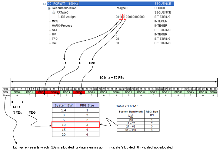
2. Resource Allocation Type 0: The Wholesale Method

Type 0 is the simplest method. Instead of assigning RBs one by one, the scheduler assigns them in Groups.

The Concept: RBG (Resource Block Group) As you learned in the previous section, we group consecutive RBs into an RBG. Important Rule: The number of RBs in a group changes based on your System Bandwidth.

System BW	Total RBs	RBG Size (How many RBs in 1 Group)
1.4 MHz	6	1
5 MHz	25	2
10 MHz	50	3
20 MHz	100	4
How it Works (The Bitmap)
In Type 0, the specific instruction sent to the phone is a bitmap, but each bit represents one RBG, not one RB.

Example (from your file): 10 MHz Bandwidth

• Total RBs: 50
• RBG Size: 3 (meaning RBs are bundled in threes: {0,1,2}, {3,4,5}…)
• Total RBGs: 17 groups (50 divided by 3, rounded up).
• The Instruction: The user receives a 17-bit bitmap. If the bitmap says 1000..., the user grabs RBG 0 (which contains physical RBs 0, 1, and 2).

Pros/Cons:

• Good: drastically reduces the message size (17 bits instead of 50).
• Bad: “Granularity” is lost. You cannot assign just RB #1. You must assign the whole group (0, 1, 2) or nothing.

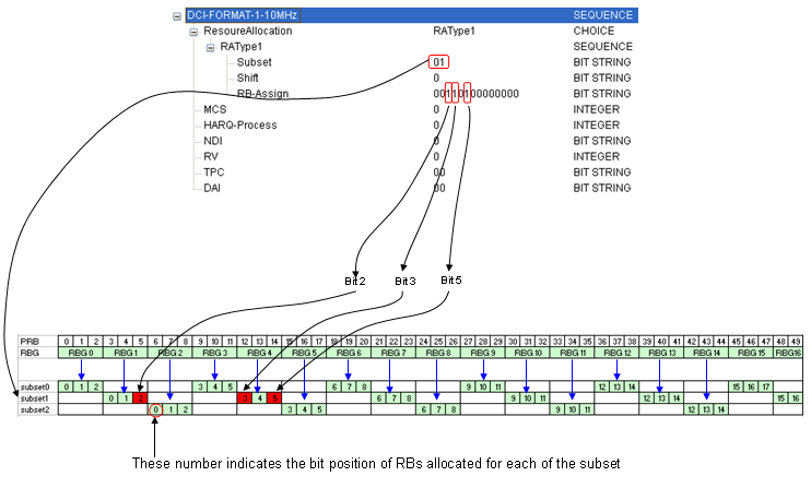
3. Resource Allocation Type 1: The “Scattered” Method

The document notes that explaining this without a picture is hard, so let’s break it down conceptually. Type 1 is designed to support Frequency Diversity.

Sometimes, the channel quality is bad in one spot but good in another. You might want to give a user RB #0 (low freq), RB #10 (mid freq), and RB #48 (high freq) to ensure some data gets through. Type 0 (Grouping) makes this hard because it forces you to take chunks.

The Hierarchy Type 1 adds a new layer called the RBG Subset.

• Hierarchy: RB $\to$ RBG $\to$ RBG Subset.
• The number of subsets is equal to the number of RBs within a RBG.
• Instead of giving you a bitmap of all groups, the scheduler says: “I am only going to look at Subset X, and inside that subset, I will give you a bitmap of specific RBs.”

Why use this? This allows the scheduler to address individual RBs (high precision) but only within a specific scattered subset of the total bandwidth. It saves bits by not addressing the whole bandwidth at once.

Note: In practice, Type 1 is complex and less commonly discussed in basic optimization compared to Type 0 and Type 2.

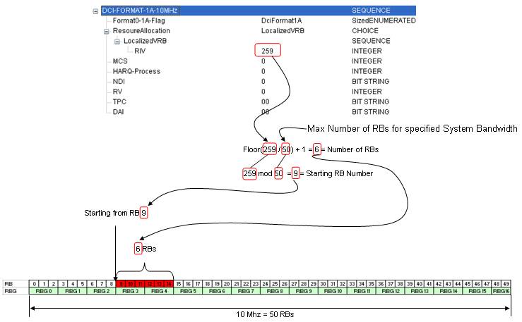
4. Resource Allocation Type 2: The “Contiguous” Method

This is a very common type. Unlike Type 0 (which allows gaps like “Group 1 and Group 5”), Type 2 forces the allocation to be Contiguous (e.g., “RBs 10 through 20”).

The Instruction Format (RIV) Because the data must be contiguous (a single block), we don’t need a bitmap. We only need two numbers:

1. Start: Where does the block begin? (e.g., RB #10)
2. Length: How long is the block? (e.g., 5 RBs)

LTE mathematically combines these two numbers into a single value called the RIV (Resource Indication Value). This is extremely efficient for message size.

Virtual vs. Physical (VRB vs. PRB) Your document highlights a critical distinction here: Virtual RBs (VRB) vs. Physical RBs (PRB).

• Virtual (Logical): The MAC layer says, “Give this user 5 contiguous RBs.”
• Physical (Reality): How do those 5 RBs actually sit on the frequency grid?

Type 2 offers two modes to handle this mapping:

A. Localized (LVRB):

• Concept: What you see is what you get.
• Mapping: Virtual RB $0,1,2$ $\to$ Physical RB $0,1,2$.
• Use Case: The scheduler knows the channel is excellent at that specific frequency.

B. Distributed (DVRB): Notes that the virtual block for this mode is still in sequence.

• Concept: The MAC layer assigns a contiguous block (Virtual 0, 1, 2), but the PHY layer scatters them across the frequency band (e.g., Physical 0, 25, 49).
• Why? This provides Frequency Diversity. If there is interference at frequency #0, you lose the first part of the data, but the parts at #25 and #49 might survive.
• Trade-off: It is more complex to calculate, but safer for users with unstable channels.